Lab 4: Observability, Reliability and Production Readiness

Overview

This final lab, which spans 2 physical sessions, focuses on making your Logic Service production-ready: observability, reliability, optimized CI/CD and deployment quality.

Introduction

You've successfully deployed your Logic Service to Kubernetes and it's running in a competitive multiplayer environment. Now it's time to make your service production-ready by adding observability, improving reliability, and implementing best practices for continuous deployment.

This lab introduces more open-ended challenges that require independent research and problem-solving. Focus on implementing Core Requirements before moving onto the more advanced topics.

Core Requirements

• Monitoring & Observability
  • Deploy Grafana using Helm with proper configuration
  • Create enhanced resource dashboards (CPU/Memory with limits)
  • Instrument code with minimum 4 custom metrics including move_execution_time
  • Create dashboards for custom metrics
  • Document instrumentation strategy
• Pipeline Quality & Visibility
  • Add code coverage reporting and parsing to CI/CD
  • Add test result reporting
  • Achieve minimum 60% code coverage
  • Add pipeline and coverage badges
• Deployment Optimization
  • Implement GitLab CI rules to control builds/deployments
  • Configure resource limits for containers (default 256 MiB memory, 100m CPU)
• State Persistence & Reliability
  • Implement game state persistence with file-based storage
  • Add graceful shutdown hooks
  • Use Kubernetes Persistent Volumes

Advanced Challenges

• Zero-Downtime Deployments
  • Implement custom readiness probe (required) and optionally custom liveness probe
  • Configure rolling updates
  • Test and validate availability during deployments
• Alerting
  • Set up at least 2 meaningful Grafana alerts
  • Configure notifications to GitLab Alerts
  • Generate alert activity for supervisor review

For full details on the deliverables of this lab, see the Practicalities section.

Observability (Prometheus & Grafana)

In cloud-native environments like Kubernetes, services are distributed, ephemeral, and often restarted. This makes traditional debugging approaches (logging into a server, inspecting files) insufficient. Observability is the practice of instrumenting your systems so you can understand their internal state by examining their external outputs—primarily metrics, logs, and traces.

For this lab, we focus on metrics: numeric measurements captured over time that reveal system behavior and performance. Unlike logs (discrete events) or traces (request flows), metrics provide aggregatable, queryable data perfect for dashboards and alerts.

Why Observability Matters for Your Logic Service

Your Logic Service is competing in a live multiplayer environment where:

• Performance matters: Slow move calculations result in timeouts and score penalties
• Reliability is critical: Crashes or errors immediately impact your faction's standing
• Behavior evolves: As you improve your logic, you need to verify if it works as intended
• Debugging is harder: Multiple teams, shared infrastructure, and pod restarts complicate troubleshooting

Without observability, you're flying blind. With it, you can answer critical questions:

• What's broken? (The symptom: high latency, error rate spike, resource exhaustion)
• Why is it broken? (The cause: inefficient algorithm, resource contention, bugs in new logic)

This principle—distinguishing symptoms from causes—comes from Google's Site Reliability Engineering practices:

Your monitoring system should address two questions: what's broken, and why? The "what's broken" indicates the symptom; the "why" indicates a (possibly intermediate) cause. "What" versus "why" is one of the most important distinctions in writing good monitoring with maximum signal and minimum noise.

Your monitoring should provide high signal, low noise: alerting only on actionable problems while giving you enough data to diagnose root causes quickly.

Your Observability Strategy

For this lab, you will:

1. Instrument your Logic Service with custom metrics that capture application behavior
2. Deploy Grafana to visualize metrics from Prometheus (already collecting data cluster-wide)
3. Create dashboards that show both infrastructure metrics (CPU, memory) and application metrics (move latency, decision patterns)
4. Document your approach explaining what you measure and why it matters

Focus on actionable metrics tied to your faction logic:

• Latency: How long do move calculations take? Are some unit types slower?
• Throughput: How many moves per second are you processing?
• Errors: Are calculations failing? What error types occur?
• Business metrics: Gold balance over time, unit composition, territory size
• Resource usage: CPU/memory consumption correlating with game state, approaching memory limits (256 MiB default)

Think of metrics as answering questions you'd ask when debugging: "Is the service slow because of expensive Cleric path finding?" or "Did the latest deploy reduce average latency?" Your instrumentation should make these questions trivially answerable via a quick dashboard glance.

Start Simple, Iterate

Begin with the required move_execution_time histogram. Once that works, add counters for move types, gauges for resource state, and any other metrics that help you understand your logic's behavior. You'll refine your instrumentation as you see what's useful versus what's just noise.

Prometheus

Prometheus is an open-source monitoring and alerting system designed for reliability and scalability. Originally developed at SoundCloud, it's now a CNCF graduated project widely used in cloud-native environments alongside Kubernetes.

How Prometheus Works

Prometheus uses a pull-based model: it periodically scrapes (pulls) metrics from HTTP endpoints exposed by your services. This is different from push-based systems where applications actively send metrics to a central server. Your Logic Service will expose metrics at /q/metrics (Quarkus default endpoint), which Prometheus scrapes every few seconds.

Each metric consists of:

• Metric name: Describes what is being measured (e.g., move_execution_seconds)
• Labels: Key-value pairs that add dimensions (e.g., unit_type="soldier", outcome="success")
• Value: The numeric measurement
• Timestamp: When the measurement was taken

Labels are powerful—they let you slice and dice data in queries. For example, instead of creating separate metrics like soldier_moves_total and worker_moves_total, you create one metric unit_moves_total{unit_type="soldier"} and unit_moves_total{unit_type="worker"}.

Cardinality Management

Avoid using unbounded label values (like unique IDs, timestamps, or user-specific data) as this creates cardinality explosion, overwhelming Prometheus with millions of unique time series. Stick to labels with a known, limited set of values (e.g., unit types, move types, status codes).

Metric Types

Prometheus defines four metric types to represent different kinds of measurements:

1. Counter - Cumulative metric that only increases (or resets to zero on restart)

• Use for: Total number of requests, total moves executed, total errors
• Example: http_requests_total, unit_moves_total
• Query with rate() or increase() to see change over time

2. Gauge - Metric that can go up or down

• Use for: Current values like memory usage, queue size, number of active units
• Example: memory_usage_bytes, active_units, gold_balance
• Query directly without rate functions

3. Histogram - Samples observations and counts them in configurable buckets

• Use for: Request latencies, response sizes, move execution times
• Example: move_execution_seconds with buckets [0.001, 0.01, 0.1, 1.0]
• Automatically provides _sum, _count, and _bucket time series
• Use histograms for latency measurements in this lab—they enable percentile calculations

4. Summary - Similar to histogram but calculates quantiles on the client side

• Less common; histograms are preferred for most use cases
• Use only when you need pre-calculated quantiles

For detailed explanations, see the Prometheus metric types documentation.

PromQL: Query Language

PromQL (Prometheus Query Language) is used to select and aggregate time series data. It's functional and expressive, designed specifically for time-series operations.

Basic query examples:

# Select all time series for a metric
http_requests_total

# Filter by labels
http_requests_total{job="logic-service", status="200"}

# Rate of requests per second (for counters)
rate(http_requests_total[5m])

# Average across all instances
avg(rate(http_requests_total[5m]))

# 95th percentile latency from histogram
histogram_quantile(0.95, rate(move_execution_seconds_bucket[5m]))

Key PromQL functions you'll use:

• rate(): Calculate per-second rate of increase (for counters)
• sum(), avg(), min(), max(): Aggregate across labels
• by (label): Group aggregations by specific labels
• histogram_quantile(): Calculate percentiles from histogram buckets

Learn PromQL

Read these official guides before continuing:

1. PromQL Basics
2. PromQL Query Examples

We'll walk through practical PromQL queries when you set up Grafana dashboards.

What You'll Do in This Lab

For your Logic Service, you will:

• Instrument your code using Micrometer (Quarkus's metrics library with Prometheus integration)
• Expose metrics at /q/metrics endpoint (automatically configured)
• Create custom metrics including move_execution_time histogram with labels for unit types
• Use meaningful labels (e.g., unit_type, move_type, outcome) instead of creating many metric names
• Query metrics with PromQL to build visualizations and alerts in Grafana
• Aggregate across pod restarts using appropriate PromQL queries to handle pod life cycle

Your metrics should focus on application behavior: move execution latency, decision patterns, resource allocation, errors, and game-specific logic. Kubernetes already provides infrastructure metrics (CPU, memory) via built-in exporters.

DevOps Cluster Setup

For this course, Prometheus is already deployed and configured on the shared Kubernetes cluster. You don't need to install or manage a Prometheus instance. Your Logic Service just needs to expose metrics, and Prometheus will automatically discover and scrape them via Kubernetes service discovery.

You'll access Prometheus data through Grafana for querying and visualization.

Grafana

Grafana is an open-source dashboarding, analytics, and monitoring platform that is tinkered for connecting with a variety of sources like Elasticsearch, Influxdb, Graphite, Prometheus, AWS Cloud Watch, and many others.

Grafana invests heavily in these data source integrations with almost every other observability tool out there. It allows you to use one product for metrics, another for logging, and a 3^rd for tracing, and bring it all together with the Grafana UI.

In our case, we are going to focus on visualizing the metrics data from Prometheus, to gain insight in the operation of our Logic Service.

If you are interested to learn more about Grafana after this lab, maybe to set it up on your home server, they have well written and extensive tutorials on various topics here.

Installing Grafana

We are going to deploy Grafana in our team namespace and we are going to use helm to do this.

Helm is a package manager for Kubernetes, it is the easiest way to find, share, and use software built for Kubernetes. Helm is a tool that streamlines installing and managing Kubernetes applications. Think of it like apt/scoop/homebrew for Kubernetes.

Helm uses a packaging format called charts. A chart is a collection of files that describe a related set of Kubernetes resources. A single chart might be used to deploy something simple, like a memcached pod, or something complex, like a full web app stack with HTTP servers, databases, caches, and so on.

Install Helm on your local machine by following the instructions on the Helm website.

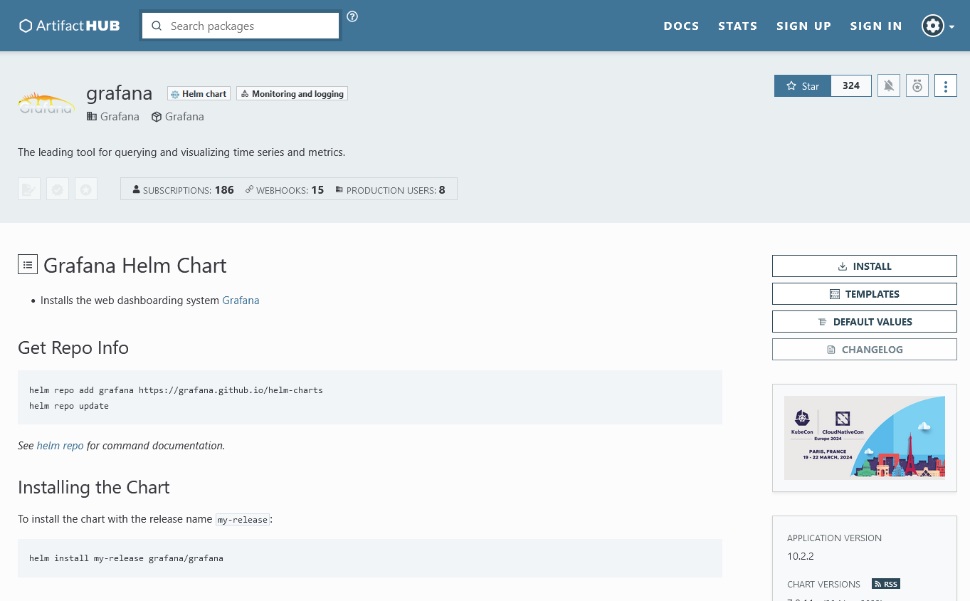
To find the Grafana Helm chart go to ArtifactHub, a web-based application that enables finding, installing, and publishing Kubernetes packages. You can discover various applications here, either as Helm charts, Kustomize packages or Operators. Search for the official Grafana chart and open it up (the one owned by the Grafana organization).

ArtifactHub provides a nice and user-friendly view on the source code of the chart, which is hosted on a Git repository (you can always navigate to that through Chart Source link in the right side bar). The chart homepage shows the readme, commonly this houses some getting started commands, changelog and a full configuration reference: table of all possible values that can be set. ArtifactHub also provides dialogs for Templates, Default Values and Install.

If you open up Templates you will see that this chart deploys quite a lot of different resources. That is the beauty of using a tool like Helm to install and manage Kubernetes applications. Instead of manipulating all these resources separately and having to keep track of them manually, everything is packaged into a release. Helm makes it easy to test out new third party applications on your cloud environment, because when you are done testing you can easily helm uninstall the release and you are left with a clean cluster.

To get started, follow the Get Repo Info instruction on the readme to add the Grafana repository to your local list of repos.

To configure our installation of the Grafana chart we can either use --set parameters when installing the chart, or preferably in this case we can make a values file to override the chart's defaults.

Navigate to your project's root folder and make a new subfolder monitoring. In this folder we are going to create a new file and call that grafana-values.yaml. This file will hold all the values we want to override in the Grafana chart, when we refer to values we mean the configuration values that be seen either in the Configuration section of the chart's readme, or in the Default Values view on ArtifactHub.

Admin password

First of all, we need to set a password for our admin. If we do not set it, Grafana will auto generate one and we will be able to retrieve it by decoding a secret on the Kubernetes cluster. However, every time we would upgrade our release, Grafana would again generate a new secret, sometimes resetting the admin password. That is why we will override it using our own secret. The Grafana chart allows you to configure your admin credentials through a secret, via admin.existingSecret and its sibling values.

NOTE: it is very important to use a strong password, we are going to expose Grafana on a public URL and we do not want trespassers querying our Prometheus server.

Add a secret to store your admin username and password

REQUIRED: Create a secret called grafana-admin with exactly these key names:

• Key: admin-user → your chosen username
• Key: admin-password → your chosen strong password

These exact names are required for Grafana to read the credentials correctly!

Creating the secret:

kubectl create secret generic grafana-admin \
  --from-literal=admin-user=<your-username> \
  --from-literal=admin-password=<your-strong-password>

Generate a strong password (required - Grafana will be publicly accessible):

# Unix/Linux/macOS - generates random 32 character password
< /dev/urandom tr -dc _A-Z-a-z-0-9 | head -c${1:-32};echo;

Use a password manager to store these credentials securely!

Configure Grafana to use the secret:

After creating the secret, add these values to your grafana-values.yaml to reference it:

admin:
  existingSecret: grafana-admin
  userKey: admin-user
  passwordKey: admin-password

Check the Grafana Helm Chart documentation for more details.

Fallback (not recommended): If you cannot get the secret working, you can use --set admin.password=<strong-password> in your Helm install command, but you will lose points for not using Kubernetes secrets properly!

Ingress Rules

In order to easily reach our Grafana UI, we are going to serve it on a path on our public domain https://devops-proxy.atlantis.ugent.be

To achieve this, we have to add Ingress to Grafana. If you search for the keyword ingress on the Values dialog, you will find that there are a bunch of variables that we can set to configure it.

We are going to serve Grafana on a path, the path being /grafana/devops-team<number>, making our dashboard accessible at https://devops-proxy.atlantis.ugent.be/grafana/devops-team<number>.

The readme of the chart has an example on how to add a ingress with path (Example ingress with path, usable with grafana >6.3), use that example and change it appropriately! This is how we work with third party charts. Read the readme for instructions and adapt it to your situation.

Disabling RBAC and PSP

The Grafana chart deploys some Role Based Access Control (RBAC objects) and Pod Security Policies by default. We won't be needing these resources so add the following to disable these options. Not disabling these will throw errors on installations because your devops-user accounts linked to your kubeconfig are not allowed to create RBAC and Security Policies.

rbac:
  create: false
  pspEnabled: false
serviceAccount:
  create: false

First Grafana release

Before moving on to the actual installation let's perform a dry-run to make sure everything is in order. A dry-run is a Helm command that simulates the installation of a chart, it will render the templates and print out the resources that would be created. This is a good way to check if your values file is correct and if the chart is going to be installed as you expect.

helm install grafana grafana/grafana -f grafana-values.yaml --dry-run

If you get a print out of all resources and no errors, you are good to go. Open up a second terminal: here we will watch all kubernetes related events in our namespace:

kubectl get events -w

Now install the Grafana helm chart:

helm install grafana grafana/grafana -f grafana-values.yaml

You will see that kubernetes creates deployments, services, configmaps and other resources in the events. The kubectl get events instruction is nice to use while learning the ropes of Kubernetes, because it can give you lots of insight into the moving parts.

When we install the chart, the helm command gives us a printout of the Helm Charts NOTES.txt file. In this file chart owners can specify some guidelines and next steps for users.

Here they guide you through retrieving the admin password (referring to a secret called grafana-admin which was created before we installed the chart and specified in the grafana-values.yaml file), and provide some extra info. This info is generated and can be different for each release because it is based on the values we set in our grafana-values.yaml file. Sadly it often contains some errors, like in the example below they claim the outside URL is http://devops-proxy.atlantis.ugent.be while it is actually http://devops-proxy.atlantis.ugent.be/grafana/devops-team0. And while it does tell you how to retrieve the admin password, it claims that you can log in with the admin username (the default), while we have set up our own admin username in a secret.

NAME: grafana
LAST DEPLOYED: Thu Nov 28 11:17:38 2024
NAMESPACE: devops-team0
STATUS: deployed
REVISION: 1
NOTES:
1. Get your 'admin' user password by running:

   kubectl get secret --namespace devops-team0 grafana-admin -o jsonpath="{.data.admin-password}" | base64 --decode ; echo


2. The Grafana server can be accessed via port 80 on the following DNS name from within your cluster:

   grafana.devops-team0.svc.cluster.local

   If you bind grafana to 80, please update values in values.yaml and reinstall:

    securityContext:
    runAsUser: 0
    runAsGroup: 0
    fsGroup: 0

    command:
    - "setcap"
    - "'cap_net_bind_service=+ep'"
    - "/usr/sbin/grafana-server &&"
    - "sh"
    - "/run.sh"

   Details refer to https://grafana.com/docs/installation/configuration/#http-port.
   Or grafana would always crash.

   From outside the cluster, the server URL(s) are:
     http://devops-proxy.atlantis.ugent.be

3. Login with the password from step 1 and the username: admin
#################################################################################
######   WARNING: Persistence is disabled!!! You will lose your data when   #####
######            the Grafana pod is terminated.                            #####
#################################################################################

Remember the command to retrieve your admin password and decode it. If you would ever forget the Admin password, or if you used a really strong password as you should, you can run that command to retrieve your admin password and copy it.

Now inspect your namespace using kubectl, finding answers to the following questions:

• Are there any pods running?
• Has a service been deployed?
• Is there an ingress resource?

When all is clear, and your Grafana pods are running, you can visit https://devops-proxy.atlantis.ugent.be/grafana/devops-team<your-team-number> on a browser and login with the admin credentials. Once logged in, you will see the Home screen of your Grafana installation.

Browser Cache Issue

On first visit, use incognito mode or disable cache! The domain root (devops-proxy.atlantis.ugent.be) hosts the game UI, and browser redirects can sometimes interfere with the Grafana path (/grafana/devops-team<X>).

If you get redirected to the game UI instead of Grafana:

• Open the URL in incognito/private browsing mode, OR
• Clear your browser cache for the domain, OR
• Hard refresh (Ctrl+Shift+R / Cmd+Shift+R)

After the first successful login, normal browsing works fine.

Adding persistence to Grafana

The Grafana Chart developers warned us about something in their NOTES.txt file:

#################################################################################
######   WARNING: Persistence is disabled!!! You will lose your data when   #####
######            the Grafana pod is terminated.                            #####
#################################################################################

Before we start making dashboards we have to add some persistence to Grafana. Default deployed Kubernetes applications have ephemeral storage, meaning that when the pod gets restarted, it is an entirely new entity and it has lost all its data (save for those fed from Secret or ConfigMaps).

So it is possible to store certain things to disk, inside the container, but these will not be persisted and survive any form of restart. Therefore we are going to mount a volume into our Grafana application which can survive restarts. The Helm chart for Grafana already has values for us to fill out.

If we go back to the Grafana Values page and search for the keyword persistence we find a number of variables to fill out. We will only be needing the following:

persistence:
  enabled: true
  size: 1Gi
  storageClassName: k8s-studstorage

So we enable persistence, request a volume with size of 1Gi and tell Kubernetes to use the storage class k8s-studstorage. Add this yaml snippet to your existing grafana-values.yaml.

These storage classes enable something called Dynamic Volume Provisioning.

Dynamic volume provisioning allows storage volumes to be created on-demand. Without dynamic provisioning, cluster administrators have to manually make calls to their cloud or storage provider to create new storage volumes, and then create PersistentVolume objects to represent them in Kubernetes. The dynamic provisioning feature eliminates the need for cluster administrators to pre-provision storage. Instead, it automatically provisions storage when it is requested by users.

Before upgrading our Grafana helm release, go ahead and open up a second terminal, in this terminal we will again watch all kubernetes related events in our namespace:

kubectl get events -w

Now from our terminal in the monitoring work directory, upgrade your grafana Helm release, with your updated grafana-values.yaml file.

As you see in the events logs, a new pod gets created for Grafana, because through setting persistence, its config is changed and it now has a volume to attach.

The chart will have created a Persistent Volume Claim (look for it using kubectl get pvc) which holds the configuration of the volume: storage class, size, read/write properties etc. This PVC then gets picked up by our storage provisioner (to which we linked by defining the storage class name) who provisions the volume.

This volume is then represented by a Persistent Volume (kubectl get pv will show you not only volumes in your namespace, but all volumes across the cluster).

While all this storage provisioning goes on our new pod is Pending, waiting for the volume to come available. When it becomes available the images get pulled and the new pod gets created. When the Grafana pod is Ready, the first pod gets killed.

Notice we now have upgraded Grafana with no downtime!

Adding Users

It is best to not use the Admin account for normal operation of Grafana, instead we use our own personal user accounts. These still need to be added and/or invited by the Admin, so that is what we are going to do next.

Log in using the admin credentials, in the left navigation bar, go to Administration>Users then to Organization Users.

You'll see one user already, the admin. Now click on Invite to start inviting team members. Add their email in the first field and leave Name open. What permission you give to each member is entirely up to you. Viewers can only view dashboards, Editors can create and edit dashboards and Admins can change settings of the Server and the Organization. You can change user permissions later as well.

Since we don't have a mailing server set up with Grafana we can't actually send the invitation email, so deselect the Send invite email toggle

When you Submit a user, you can navigate to Pending Invites and click Copy Invite to retrieve the invite link. Now send that invite link to the appropriate team member, or open it yourself.

When you follow your invite link, you can set username, email, name and password yourself.

Adding a Data Source

If we want to make dashboards, we are going to need data. On the Home screen of your Grafana you can see a big button Add your first data source, click it or navigate to Connections>Add new connection.

We are going to link to the Prometheus server that has already been set up in the prometheus namespace. Select Prometheus from the list of Data Sources.

Enter the following URL to point your Grafana instance to the already deployed Prometheus server:

http://prometheus-operated.monitoring:9090

Leave everything else on its default. Click Save & Test at the bottom of your screen. If all went well you should get a green prompt that your Data Source is working.

Exploring the data

The Prometheus instance we are running, collects a lot of data regarding the resource usage of our containers as well as multiple Kubernetes related metrics and events such as pod restarts, ingress creations, etc.

If you want to explore the data and build queries, the best place to go is the Explore screen on Grafana (compass in the navigation bar).

Tip

Grafana defaults to a Builder view to construct your query. This tool is very handy to start building your own queries and even get feedback on what each piece of the query does when enabling the Explain toggle at the top.

The raw query gets shown by default and can also be toggled if wanted.

The following introduction however uses the Code view to construct our query. Follow along with the Code view first and then you can move back to the Builder view.

For instance, let's say we are interested in CPU, when you type in cpu in the query bar at the top, it will auto complete and show a list of matching suggestions. Hovering over any of these suggestions will give you the type of metric and a description.

If we select container_cpu_usage_seconds_total you will see that we can actually select an even more specific metric if we want to.

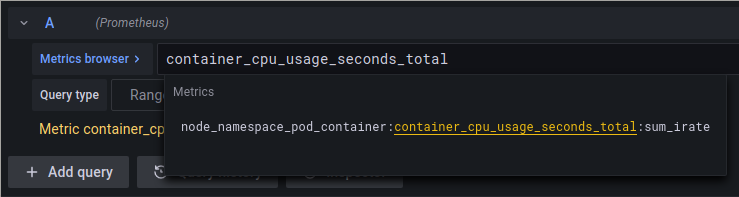
These prefixes and suffixes indicate that these metrics were made by special recording rules within Prometheus. These rules are often much easier to work with because they have already filtered out certain series and labels we aren't interested in.

node_namespace_pod_container:container_cpu_usage_seconds_total:sum_irate

node_namespace_pod_container indicates that these metrics have those four labels available, we can use these to filter our query.

sum_irate indicates that these metrics have already been applied both the sum and irate function.

When we click Run Query we will get a lot of metrics, one for each container in the cluster, across all namespaces. We are only interested in our own namespace of course!

Warning

While we encourage trying out PromQL and Grafana, please take the following in mind:

• You may query data from other namespaces for academic purposes, to get the hang of the PromQL query language and basic monitoring. It is however not allowed to scrape and process metrics from the namespaces of other teams with the intent to extract Operational information from their logic.
• When experimenting with queries, set the range to fifteen minutes, one hour max. When you have filtered your query enough so that it doesn't return millions of irrelevant fields, you can expand this range to the required value for observability. Repeated queries over large time ranges, on series with lots of fields will negatively impact the performance of both your Grafana service and the Prometheus server. Prometheus queries can be backtraced to its origin.

Now we will add our first selector to our PromQL query. First, let us narrow our query to all pods in our namespace. Open curly brackets at the end of your selector, notice that Grafana prompts you with the available options for labels:

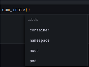
Go ahead and select only the metrics from your own namespace. You will see two series have been selected. One for our Logic Service container and one for Grafana. Now add another selector to the list so that you only query the CPU usage of your Logic Service. We will use this query in the next step so copy it or keep it handy.

Tip

You can create this same query using the builder, it will show a blue box with hint: expand rules(). The metric we are querying is what's called a Recording rule. A Prometheus query that is continually run in the background by Prometheus, the results of this query are then recorded as another metric. Go ahead and expand the rule, you will see the raw query and by enabling the Explain toggle will also get some info about them.

You can keep on using the builder or the code view for your own queries, the choice is up to you. The explain toggle is a handy tool to learn PromQL hands-on.

Now that you can query metrics, let's understand what constraints your Logic Service operates under before building dashboards.

Understanding Resource Limits

Before creating dashboards, it's important to understand the resource constraints your Logic Service operates within. The cluster has resource quotas and limits configured for your namespace to ensure fair resource distribution among all teams.

Default Resource Configuration:

• Memory Request: 256 MiB (guaranteed allocation)
• Memory Limit: 256 MiB (hard cap, pod will be OOMKilled if exceeded)
• CPU Request: 100m (0.1 CPU cores, guaranteed)
• CPU Limit: None (can burst to available capacity)

Kubernetes Best Practices

Following Kubernetes best practices:

• Memory: Request = Limit prevents memory overcommit and ensures predictable behavior
• CPU: Request without limit allows bursting during high load while guaranteeing minimum capacity

This configuration balances performance with resource efficiency.

If your Logic Service needs more memory (e.g., for complex pathfinding or state caching), you can request up to 512 MiB maximum by adding resource specifications to your deployment.yaml:

spec:
  template:
    spec:
      containers:
        - name: logic-service
          image: ...
          resources:
            requests:
              memory: "384Mi" # Adjust as needed (256-512 MiB)
              cpu: "100m" # Minimum guaranteed
            limits:
              memory: "384Mi" # Must match request
              # No CPU limit - allows bursting

JVM Memory Tuning

Your Logic Service runs on JRE 25 which is container-aware and automatically detects memory limits. For small containers (256-512 MiB), you may want to tune heap allocation:

env:
  - name: JAVA_OPTS
    value: "-XX:InitialRAMPercentage=50.0 -XX:MaxRAMPercentage=75.0"

This sets max heap to 75% of container memory, leaving room for off-heap (threads, code cache). Adjust if you see OOMKills or want different heap behavior.

Observe First, Tune Later

JVM defaults work well for most cases. Only tune after observing memory behavior in Grafana and pod logs (kubectl logs).

JVM Metrics Available: Quarkus automatically exposes JVM-specific metrics at /q/metrics including heap usage, GC activity, and thread counts. Explore these in Prometheus to understand memory behavior before tuning.

See JDK Ergonomics for advanced tuning options.

Memory Limit = OOMKill

If your container exceeds its memory limit, Kubernetes will immediately kill the pod (Out Of Memory Kill). This appears as pod restarts in your deployment. Monitor memory usage closely!

Memory approaching its limit is an excellent alerting condition. In the Advanced section on Alerting, you'll set up alerts that trigger when memory usage crosses thresholds (e.g., 80% of limit). This gives you early warning before OOMKills occur.

Creating a Dashboard

Now that you understand your resource constraints, let's create a dashboard to visualize them. When we visit our Home screen again now, we can see we have completed adding our first Data Source. Next to that button, Grafana is prompting us to add our first dashboard.

Either click the big button on your Home screen or navigate to Dashboards>New Dashboard.

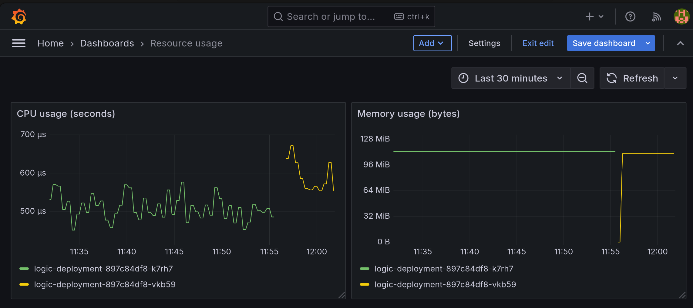
Now you have a completely empty dashboard. We will get you going by helping you create simple panels to visualize CPU and Memory usage of our logic-service.

Click on Add Visualisation and copy your previous CPU query in the Metrics section and give your panel an appropriate name. You'll see that your series will have a very long name in the legend on the bottom of the graph. Default it will show the metric name plus all its labels. We can actually use these labels to override the legend, setting {{pod}} as legend format, will change the legend name to only the pod name.

Info

If you use the code view you might see warning to apply a rate() function which you can safely ignore. The recording rule has already applied the rate function, but since the metadata of the metric still says it is a COUNTER type, Grafana keeps showing the warning.

Hit Save in the topright corner, you will get a dialog prompting you to give your Dashboard a name, optionally putting it into a folder. Give it a name and Save. You can always go to Dashboard settings to change the name later.

Every time you save your dashboard, you will also be asked to give an optional description. Grafana dashboards are versioned, a bit like Git, allowing you to describe changes as you go and revert some changes when needed.

Next we will add a graph to show us our memory usage. Click on Add Panel in the top bar then Add New Panel.

When you go to the Explorer again and type in memory, you can see there are a lot of options. You might think that memory utilization of our service is easily tracked with container_memory_usage_bytes, however, this metric also includes cached (think filesystem cache) items that can be evicted under memory pressure. The better metric is container_memory_working_set_bytes.

This metric also has a recording rule, similar to our previous cpu metric! Use that metric to construct your memory usage query. Apply correct label filters to only show the memory usage of your Logic Service!

Now, your legend is probably showing that you are using about X Mil or K. This is not very readable ofcourse. On the rightside panel, we can navigate to the Standard Options tab and change our Graph's unit. Alternatively you can use the Search field at the top of the rightside panel and search for "unit". Select the Data / bytes(IEC) unit.

You can also do the same for CPU usage, changing the unit to Time / seconds.

When you are happy with your graph panel, hit apply. You now see two panels, you can drag and drop these panels into any position you prefer and resize them.

Grafana can automatically refresh the data and keep things up to date, in the top right corner you can click the refresh button manually or select one of the auto refresh options from the dropdown menu. Don't forget to Save your menu, you will also get the option to save your current time range as a dashboard default (this includes any auto refresh config).

You should end up with a dashboard that looks something like this:

Enhanced Resource Dashboard with Requests/Limits

Now we have a basic dashboard and you understand resource limits and requests, create an improved resource dashboard that provides complete visibility into your container's resource usage. Focus on getting the content right, copy layout and styling for full credit:

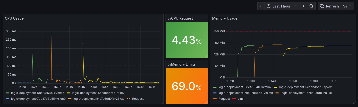
Required panels:

1. CPU Usage panel (time series):

   • Query: Current CPU usage
   • Query: CPU request line
   • Unit: seconds
   • Style request line: dashed, orange color, thicker line width

2. CPU Request Percentage panel (stat/gauge):

   • Calculate: (current CPU usage) / (CPU request) as percentage
   • Add color thresholds: green (0-40%), yellow (40-60%), orange (60-80%), red (80%+)
   • Unit: percentunit
   • Display as single stat, color the value, graph in background

3. Memory Usage panel (time series):

   • Query: Current memory usage
   • Query: Memory request line
   • Query: Memory limit line
   • Unit: bytes (IEC)
   • Style request line: dashed, orange color, thicker line width
   • Style limit line: dashed, red color, thicker line width

4. Memory Limit Percentage panel (stat/gauge):

   • Calculate: (current memory) / (memory limit) as percentage
   • Add color thresholds: green (0-40%), yellow (40-60%), orange (60-80%), red (80%+)
   • Unit: percentunit
   • Display as single stat with colored background

Instrumenting our logic service

In this section we will show you how you can create custom metrics for your application that can be picked up by Prometheus. Application-specific metrics can be an invaluable tool for gaining insights in your application, especially if you can correlate these with generic metrics (such as CPU and memory) to spot potential issues.

Quarkus provides a plugin that integrates the Micrometer metrics library to collect runtime, extension and application metrics and expose them as a Prometheus (OpenMetrics) endpoint. See the Quarkus documentation for more information.

Start by adding a new Maven dependency to the POM of your project:

<dependency>
    <groupId>io.quarkus</groupId>
    <artifactId>quarkus-micrometer-registry-prometheus</artifactId>
</dependency>

After refreshing your dependencies and starting the logic-service, you should see that Micrometer already exposes a number of Quarkus framework metrics at http://localhost:8080/q/metrics.

First instrumentation: move execution time

Micrometer has support for the various metric types we mentioned before (Counter, Timer, Gauge) and extended documentation is provided via their webpage. As an example, we will show you how you can add instrumentation for monitoring the execution time of your unit logic! We will use a Timer to measure this!

First, inject the Micrometer MeterRegistry into your FactionLogicImpl, so you can start recording metrics:

@Inject
MeterRegistry registry;

Next, wrap the implementation of nextUnitMove using Timer.record, for example:

@Override
public UnitMove nextUnitMove(UnitMoveInput input) {
    return registry.timer("move_execution_time")
            .record(() -> switch (input.unit().type()) {
                case PIONEER -> pioneerLogic(input);
                case SOLDIER -> soldierLogic(input);
                case WORKER -> workerLogic(input);
                case CLERIC -> moveFactory.unitIdle(); // TODO: extend with your own logic!
                case MINER -> moveFactory.unitIdle(); // TODO: extend with your own logic!
            });
}

This records the execution time of the unit move logic and makes sure this data can be exposed towards Prometheus. However, we also want to differentiate between the execution times of our different units' logic. Instead of creating different Timers we can add a label!

registry.timer("move_execution_time", "unit", input.unit().type().name())

Restart the logic-service and visit http://localhost:8080/q/metrics again and make sure the devops-runner is active to run a local game. The metric you've added should then be visible in the response, e.g.:

# HELP move_execution_time_seconds_max
# TYPE move_execution_time_seconds_max gauge
move_execution_time_seconds_max{unit="SOLDIER",} 2.466E-4
move_execution_time_seconds_max{unit="WORKER",} 2.026E-4
move_execution_time_seconds_max{unit="PIONEER",} 2.197E-4
# HELP move_execution_time_seconds
# TYPE move_execution_time_seconds summary
move_execution_time_seconds_count{unit="SOLDIER",} 264.0
move_execution_time_seconds_sum{unit="SOLDIER",} 0.0095972
move_execution_time_seconds_count{unit="WORKER",} 656.0
move_execution_time_seconds_sum{unit="WORKER",} 0.0381238
move_execution_time_seconds_count{unit="PIONEER",} 4274.0
move_execution_time_seconds_sum{unit="PIONEER",} 0.0929189

Changing the metrics endpoint

Right now, the metrics are exposed on the main HTTP server, at port 8080. This is not ideal, as we want to keep the main HTTP server as lightweight as possible and reserve it solely for the game logic. Therefore, we will change the metrics endpoint to a different port.

To do this all we need is to enable the management interface of Quarkus by setting quarkus.management.enabled=true in our application.properties file. This will expose a new HTTP server on port 9000, which will serve the metrics at /q/metrics.

Verify this works by visiting http://localhost:9000/q/metrics while your Logic Service is running. Make sure the devops-runner is active to generate some game moves—this will populate your metrics with actual data.

Now that your instrumentation is in place, let's test it thoroughly before deploying to Kubernetes.

Local Testing with Prometheus and Grafana

Before deploying your instrumented Logic Service to Kubernetes, it's highly recommended to test your metrics locally. This allows you to verify that your custom metrics are being exposed correctly and can be scraped by Prometheus, without the complexity of debugging in the cluster.

We can repurpose what we've learned in the Docker tutorial to set up a local Prometheus + Grafana stack using Docker Compose. This setup will scrape metrics from your locally running Logic Service and allow you to create dashboards in Grafana to visualize your custom metrics.

Testing Workflow:

1. Instrument your code with custom metrics
2. Run Logic Service locally (./mvnw quarkus:dev)
3. Start local Prometheus + Grafana with Docker Compose
4. Start the devops-runner to simulate a game and generate metrics
5. Query metrics in Prometheus and create test dashboards in Grafana
6. Once verified, deploy to Kubernetes

Setting up a Local Monitoring Stack

1. Start your Logic Service in dev mode

./mvnw quarkus:dev

Your service will run on localhost:8080 and expose metrics at http://localhost:9000/q/metrics (management port).

1. Start the devops-runner

Either run the devops-runner compose file in a separate terminal or in detached mode:

docker compose up -d

Configure the runner to your liking, a long running game is preferred in this exploration phase.

The runner will call your Logic Service's move endpoints, causing your instrumented metrics to be updated with real data.

1. Create monitoring configuration files

Create a monitoring/local folder in your project root with two files:

monitoring/local/prometheus.yml:

global:
  scrape_interval: 15s

scrape_configs:
  - job_name: "logic-service-local"
    static_configs:
      - targets: ["host.docker.internal:9000"] # Docker Desktop, linux workaround
        # - targets: ['172.17.0.1:9000']        # Docker engine alternative
    metrics_path: "/q/metrics"

monitoring/local/compose.yml:

configs:
  prometheus_cfg:
    file: ./prometheus.yml

services:
  prometheus:
    image: prom/prometheus:v3.6.0
    configs:
      - source: prometheus_cfg
        target: /etc/prometheus/prometheus.yml
    volumes:
      - prometheus-data:/prometheus
    ports:
      - 9090:9090
    extra_hosts:
      - "host.docker.internal:host-gateway" # Linux only

  grafana:
    image: grafana/grafana:12.2.0
    ports:
      - 3000:3000
    volumes:
      - grafana-data:/var/lib/grafana

volumes:
  prometheus-data:
  grafana-data:

Using Docker Compose Configs

The configs: section references files relative to the compose file location. This means you can run docker compose from anywhere:

# From project root
docker compose -f monitoring/local/compose.yml up -d

# Or from monitoring/local
cd monitoring/local
docker compose up -d

The Prometheus config will always be found correctly!

Docker host networking

• On Docker Desktop: Use host.docker.internal to access your host machine from Docker (also works with the Linux extra_hosts workaround)
• On Docker engine: Use 172.17.0.1 (default Docker bridge gateway) or add extra_hosts as shown
• Important: Use port 9000 (management port), not 8080!

1. Start the monitoring stack

From your project root:

docker compose -f monitoring/local/compose.yml up -d

1. Verify metrics collection

• Check metrics endpoint: Visit http://localhost:9000/q/metrics - you should see Prometheus format metrics
• Check Prometheus targets: Visit http://localhost:9090/targets - your logic-service-local should be "UP"
• Query in Prometheus: Go to http://localhost:9090/graph and try queries like move_execution_time_seconds_count
• Configure Grafana:
  • Visit http://localhost:3000 (admin/admin)
  • Add Prometheus datasource: URL = http://prometheus:9090
  • Create test dashboards and verify your custom metrics appear
  • Make sure the devops-runner is generating game moves to populate metric data

Benefits of Local Testing

• Faster iteration: No need to build images, push to registry, and deploy to cluster
• Easier debugging: View logs directly in your terminal
• Verify metric types: Ensure Counters increment, Gauges update, Histograms create buckets
• Test PromQL queries: Experiment with queries before adding to dashboards
• Check metric labels: Verify your labels are correct and meaningful
• Full control over test scenarios: Your team might get eliminated in the live cluster, stopping all metric generation. Locally, you control the devops-runner and can keep games running indefinitely while tuning instrumentation
• Test specific scenarios: Simulate edge cases, test faction behavior under different conditions, without affecting the competitive environment

Common Issues

• Metrics not appearing in Prometheus:
  • Check Prometheus logs: docker compose logs <prometheus-container>
  • Verify target is reachable: docker exec -it <prometheus-container> wget -O- http://host.docker.internal:8080/q/metrics
  • If using alternative target, make sure the Docker bridge IP or similar is correct

• No custom metrics visible:
  • Trigger the code path that increments/updates your metrics (make moves in a game)
  • Check if metrics appear at /q/metrics endpoint
  • Verify metric names don't have typos

Once you've verified everything works locally, you can confidently deploy to Kubernetes knowing your instrumentation is correct!

Deploying to Kubernetes

Now that your metrics work locally, it's time to deploy to the cluster. Your custom metrics will be automatically scraped by the cluster's Prometheus instance.

Update Deployment Configuration

The addition of the metrics port requires updating your Kubernetes deployment. Add the metrics port to your deployment.yaml file as an additional entry for the ports attribute of the logic-service container:

- name: metrics
  containerPort: 9000
  protocol: TCP

Warning

As always when working with YAML: double-check your indentations!

How Prometheus Discovers Your Metrics

The Prometheus server will automatically scrape the metrics port of any Service with appropriate labels in any namespace. This is configured through a PodMonitor object that's already deployed cluster-wide. Here's how it works:

apiVersion: monitoring.coreos.com/v1
kind: PodMonitor
metadata:
  name: devops-logic-combo-monitor
  namespace: monitoring
spec:
  namespaceSelector:
    any: true
  podMetricsEndpoints:
    - interval: 15s
      path: /q/metrics
      port: metrics
  selector:
    matchExpressions:
      - {
          key: app,
          operator: In,
          values: [logic-deployment, logic-service, logic],
        }

Verify your pod has this label and correct port name by using kubectl in case you can't query your custom metrics after deploying your changes.

Understanding Label Differences: Local vs Cluster

When querying metrics in Grafana after deployment, you'll notice label differences between local and cluster environments:

Local testing (your Prometheus):

• job="logic-service-local" (from your prometheus.yml)
• No pod/namespace labels (running on host, not in Kubernetes)
• Only your custom application metrics visible

Cluster (shared Prometheus):

• namespace="devops-team<X>" (your namespace)
• pod="logic-deployment-xxxxx" (pod name with unique suffix)
• container="logic-service" (container name)
• job="devops-logic-combo-monitor/devops-team<X>/logic-deployment" (from PodMonitor)

*Important for querying:**

When building Grafana dashboards on the cluster, you'll need to:

• Filter by namespace="devops-team<X>" to see only your metrics
• Use container="logic-service" to distinguish from other containers
• Your custom metrics (move_execution_time, etc.) will work with these labels
• Infrastructure metrics (container_memory_working_set_bytes, container_cpu_*) are also available

Finding Your Metrics in Cluster Prometheus

After deploying, use Grafana Explorer to search for your metric names. Example query:

move_execution_time_seconds_count{namespace="devops-team<X>"}

This will show your metric with all available labels. You can then refine your queries based on the actual label names Prometheus has recorded.

Custom metrics dashboard

Visualize move_execution_time

Add two graphs to your Grafana dashboard:

1. Unit move execution time: This graph should show the average time it takes for each unit type to execute its move logic. Each line in the graph should represent a different unit type, with the series labeled by the unit type. The y-axis should display time in seconds.
2. Unit move requests per second: This graph should show the average number of move requests per second for each unit type. Each line in the graph should represent a different unit type, with the series labeled by the unit type. The y-axis should display requests per second.

Ensure that the series are continuous and not disrupted by pod restarts by using appropriate aggregations.

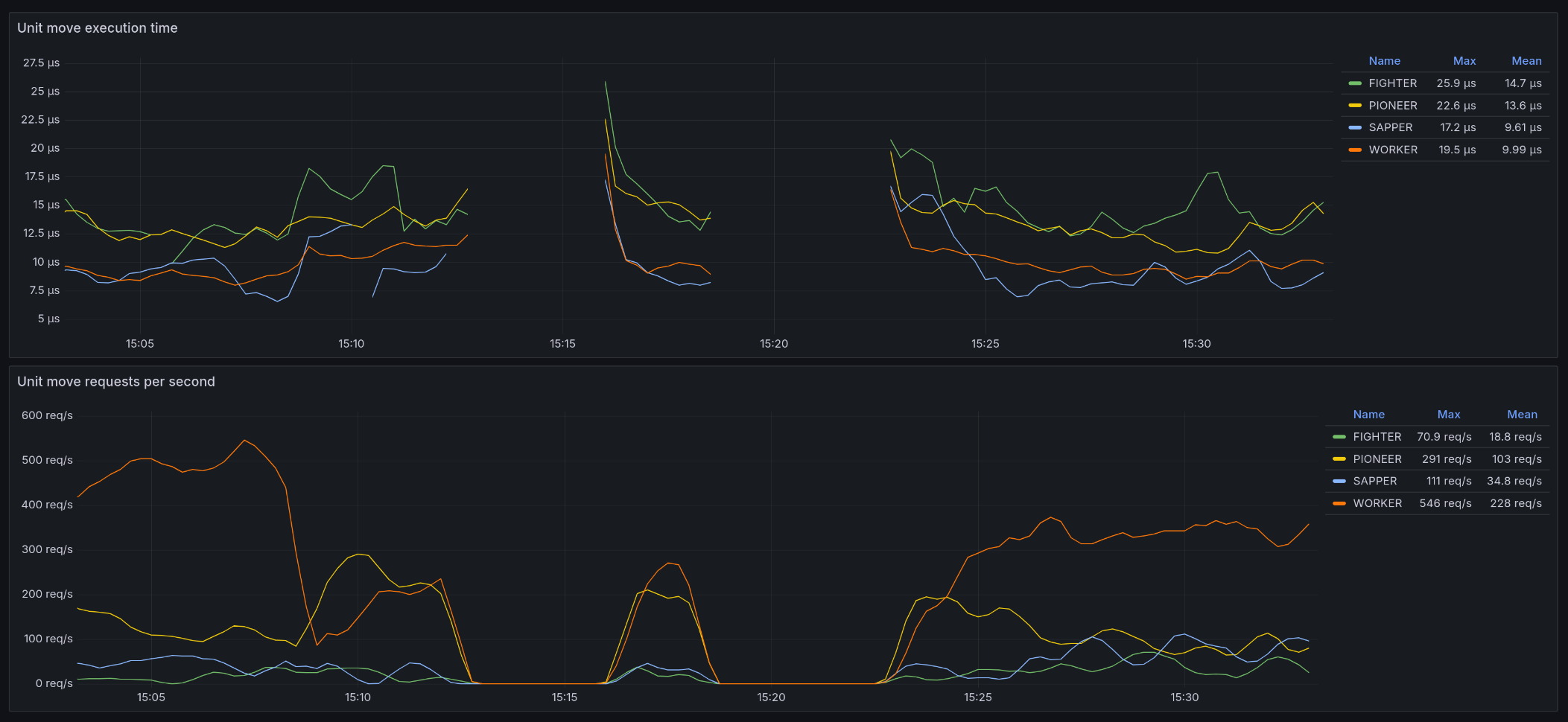
On the dashboard image above, the logic service is being restarted every 3 minutes, but the series are still continuous. The gaps in the graphs are due to the fact that the logic service is not being called because it has been defeated.

Create custom instrumentation metrics

Implement at least an additional three custom metrics for your logic service, so four custom metrics including move_execution_time. These metrics can be anything you like, but should provide insight into the performance of your logic service and faction.

More info on creating your own metrics are found here on the Quarkus Micrometer docs.

If several metrics could be represented by one metric with different labels, we will consider these as one metric for the purpose of this assignment. For example, if you have a metric worker_move_execution_time, pioneer_move_execution_time, soldier_move_execution_time, etc. these would be scored as only one metric.

Visualize these metrics on one or several Grafana dashboards. Also document the metrics (name, labels, meaning, etc.) with links to the respective dashboards, in a markdown file in the monitoring folder:monitoring/instrumentation.md. Include a link to this file in your project Report.

Experiment with the Query Builder and read through documentation of Prometheus to form your queries. To get started on visualizing the move_execution_time metric we refer to the Prometheus docs: Count and sum of observations.

General tips:

• DO NOT create different metrics that measure the same thing but for another resource, use labels!
• Make use of aggregators such as sum(), avg(), etc. Take in mind restarts of your logic service which will reset your metrics or cause disruptions in your graphs making them unreadable (see Chaos Engineering). A pod restart often results in a new series being created as the pod ID is part of the label set. This is fine for metrics like CPU / Memory because these relate to the pod itself. But for metrics that relate to the service as a whole, you want to make sure that the series are continuous.
• Make sure your dashboards are readable, both over small time ranges as big ones. Tweak year dashboards and setup proper legends, units, scales, etc. A dashboard should provide necessary information at a glance and not require extensive inspection.
• a useful tool for getting to know the PromQL language as you construct queries and explore data is the Grafana Explorer and query Builder!

Pipeline Quality (Coverage, Reports, Badges)

As we keep expanding our game logic, it is important to keep up with our testing. Therefore, we are going to add two things to our build pipeline which will help with our test visibility and most importantly: our motivation to keep writing tests.

Code Coverage Reports

Writing unit tests is not hard to do, the hardest part is getting into the habit of writing unit tests. To this end, Code Coverage reports can help motivate us.

Code coverage is a metric that can help you understand how much of your source is tested. It's a very useful metric that can help you assess the quality of your test suite. Code coverage tools will use several criteria to determine which lines of code were tested or not during the execution of your test suite.

To get these Code Coverage reports, all we need to do is add a dependency:

<dependency>
  <groupId>io.quarkus</groupId>
  <artifactId>quarkus-jacoco</artifactId>
  <scope>test</scope>
</dependency>

Now when you run mvn test and look at target folder you will see that it now has a new jacoco-report folder.

When you open the index.html browser you will be able to view and browse the report.

You can drill down from the package into the individual classes. Browsing into FactionLogicImpl gives you an overview of each element. You can then inspect these elements which gives you color coded information about your Code Coverage.

JaCoCo reports help you visually analyze code coverage by using diamonds with colors for branches and background colors for lines:

• Red diamond means that no branches have been exercised during the test phase.
• Yellow diamond shows that the code is partially covered – some branches have not been exercised.
• Green diamond means that all branches have been exercised during the test. The same color code applies to the background color, but for lines coverage.

A "branch" is one of the possible execution paths the code can take after a decision statement—e.g., an if statement—gets evaluated.

JaCoCo mainly provides three important metrics:

• Line coverage reflects the amount of code that has been exercised based on the number of Java byte code instructions called by the tests.
• Branch coverage shows the percent of exercised branches in the code – typically related to if/else and switch statements.
• Cyclomatic complexity (Cxty) reflects the complexity of code by giving the number of paths needed to cover all the possible paths in a code through linear combination.

Code Coverage parsing

GitLab has integrations built in to visualize the Code Coverage score we are now generating using jacoco. We can get our coverage score in job details as well as view the history of our code coverage score, see this particular section in GitLab Testing docs.

All this Coverage Parsing does is use a regular expression to parse the job output and extract a hit. Our mvn test does not output the total Code Coverage Score to standard out sadly. We can however extract it from the generated jacoco.csv file.

Open up your target/jacoco-report/jacoco.csv, there you will see output similar to this

GROUP,PACKAGE,CLASS,INSTRUCTION_MISSED,INSTRUCTION_COVERED,BRANCH_MISSED,BRANCH_COVERED,LINE_MISSED,LINE_COVERED,COMPLEXITY_MISSED,COMPLEXITY_COVERED,METHOD_MISSED,METHOD_COVERED
quarkus-application,be.ugent.devops.services.logic,Main,6,0,0,0,3,0,2,0,2,0
quarkus-application,be.ugent.devops.services.logic.http,MovesResource,13,0,0,0,3,0,3,0,3,0
quarkus-application,be.ugent.devops.services.logic.http,AuthCheckerFilter,18,0,4,0,4,0,4,0,2,0
quarkus-application,be.ugent.devops.services.logic.http,RemoteLogAppender,47,57,5,1,11,9,4,3,1,3
quarkus-application,be.ugent.devops.services.logic.api,BaseMoveInput,0,12,0,0,0,1,0,1,0,1
quarkus-application,be.ugent.devops.services.logic.api,UnitType,0,33,0,0,0,6,0,1,0,1
quarkus-application,be.ugent.devops.services.logic.api,BaseMoveType,0,39,0,0,0,7,0,1,0,1
quarkus-application,be.ugent.devops.services.logic.api,UnitMoveInput,18,0,0,0,1,0,1,0,1,0
quarkus-application,be.ugent.devops.services.logic.api,BonusType,0,27,0,0,0,5,0,1,0,1
quarkus-application,be.ugent.devops.services.logic.api,Location,17,43,0,0,1,14,1,7,1,7
quarkus-application,be.ugent.devops.services.logic.api,UnitMove,12,0,0,0,1,0,1,0,1,0
quarkus-application,be.ugent.devops.services.logic.api,UnitMoveType,0,87,0,0,0,3,0,1,0,1
quarkus-application,be.ugent.devops.services.logic.api,MoveFactory,136,12,0,0,18,2,18,2,18,2
quarkus-application,be.ugent.devops.services.logic.api,BaseMove,0,15,0,0,0,1,0,1,0,1
quarkus-application,be.ugent.devops.services.logic.api,Faction,0,39,0,0,0,1,0,1,0,1
quarkus-application,be.ugent.devops.services.logic.api,BuildSlotState,9,0,0,0,1,0,1,0,1,0
quarkus-application,be.ugent.devops.services.logic.api,Coordinate,27,41,5,5,2,10,7,4,2,4
quarkus-application,be.ugent.devops.services.logic.api,GameContext,0,24,0,0,0,1,0,1,0,1
quarkus-application,be.ugent.devops.services.logic.api,Unit,0,21,0,0,0,1,0,1,0,1
quarkus-application,be.ugent.devops.services.logic.impl,FactionLogicImpl,428,85,72,4,68,12,56,6,16,6

You can open up this .csv file in a Spreadsheet program to make it more readable (or use a CSV extension in VS Code). These .csv files are very easy to parse.

Extract code coverage score

Parse the jacoco.csv file using bash commands (or other scripting language of your choice) to output the total Code Coverage score (a percentage). You can limit the coverage score to the ratio of instructions covered over total instructions.

E.g.:

16.1972 % covered

Add this command/script to the test-unit job of your CI file so each test run outputs their coverage.

TIP: you can use awk. Test your command locally before adding it to your CI file.

Then construct a regular expression to capture this output and add it to your maven-test job using the coverage keyword.

You can build and test your regex using a regex tester like Regex101.

When you have added your coverage regex to your maven-test job you can push your changes to GitLab. If you then navigate to that job on GitLab, you will see your score in the Job Details

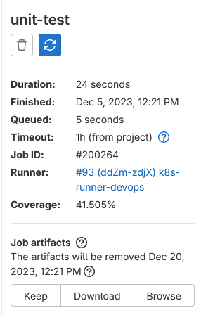
If you have an open merge request, you will also see your score in the merge request widget.

You can even start tracking your code coverage history via Analyze>Repository Analytics now.

Visualizing code coverage in MR diffs

To further improve our visibility into our code coverage, we can add some visualization to the diffs of our merge requests, using the output of jacoco to enrich the GitLab view.

TASK

Check official docs on Test Coverage Visualization and add the necessary steps to your CI file to enable this feature.

When you have set it up right, you will be able to see your code coverage in the diffs of your merge requests. Diff will show red bars for uncovered code, green bars for covered code. When there is no coverage information for a line, no bar is shown.

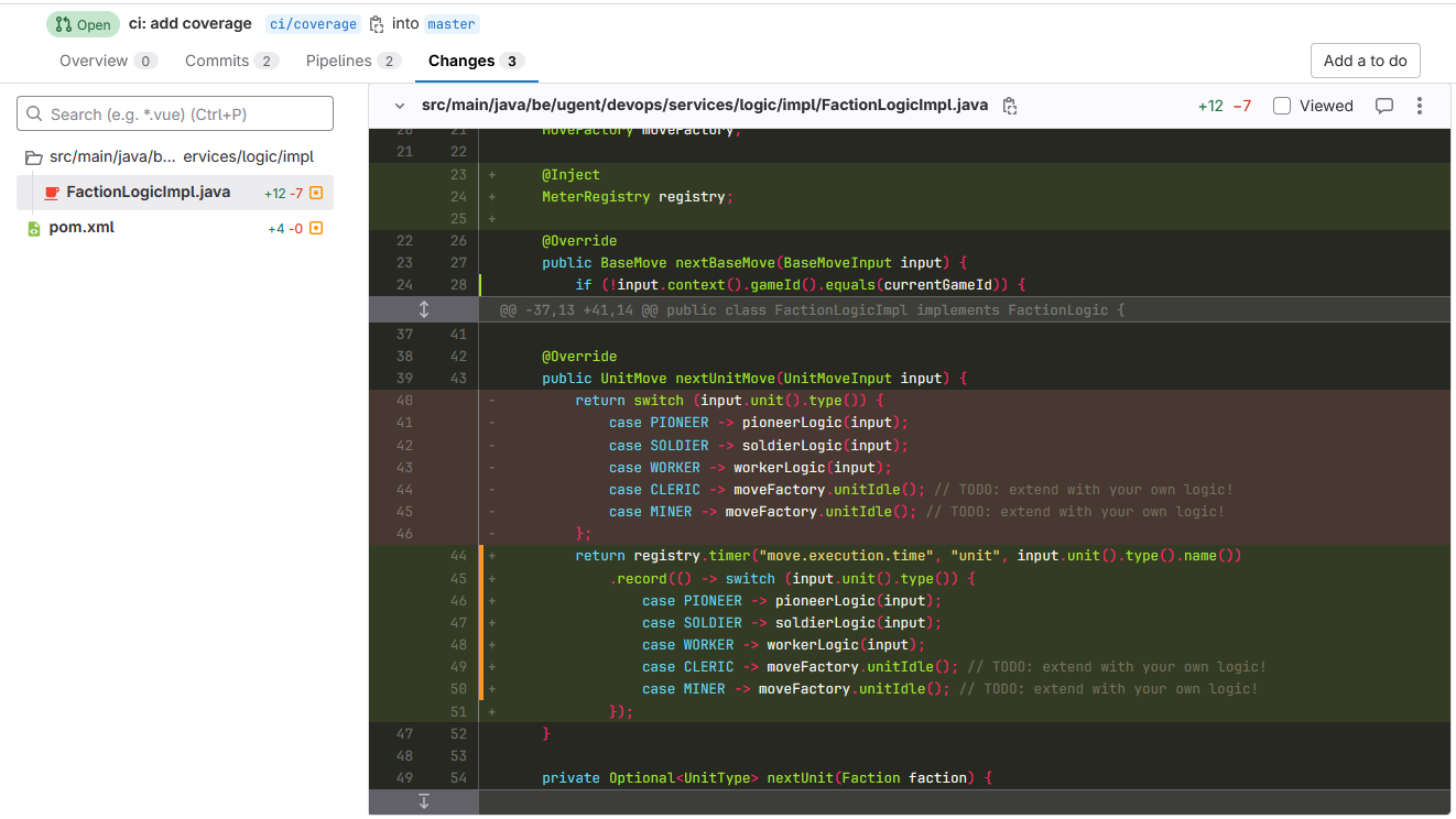
Using this and the coverage history enabled previously, you can easily check the contributions of team members and see if they are adding tests or not, pinpointing code lines that are not covered yet.

Run pipeline on merge requests

Make sure to run your pipeline on merge requests to see the coverage in the diffs. If the associated job doesn't run, the artifact isn't present and thus coverage won't be shown. See Deployment Optimization for more information.

It might take a bit of time before the coverage shows up in the diff view, GitLab needs to process the coverage report first.

Test reports in pipeline view

A final thing we can easily add is a test overview in our Pipeline view, when you go to CI/CD>Pipelines and check the details of your latest pipeline, you will notice there are tabs, one of them being Tests.

You can find instructions on the GitLab Unit Test Reports page. In our case, we are going to add the test reports to the unit-test job (View Unit test reports on GitLab).

Info

Test reports are generated by Surefire. Take a look at the target folder of your project, compare with the artifacts needed for the test report in the GitLab docs and adapt the code example!

When you have set it up right, you will be able to see all your tests in the pipeline view.

Improving test coverage

TASK

Add tests to improve your Code Coverage, aim for at least 60%. Use your Code Coverage report to get insight into what can be improved.

Do note: 100% code coverage does not necessarily reflect effective testing, as it only reflects the amount of code exercised during tests, but it says nothing about tests accuracy or use-cases completeness. To this end, there are other tools that can help like Mutation Testing, an example being PiTest which also has a Maven plugin. Implementing this is beyond the scope (and allotted time) of this course.

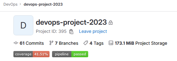
Badges

By now you must have noticed how broad of a topic DevOps really is. There is a lot at play in setting up a good automated CI/CD pipeline. However, once in place, the benefits are well worth the effort. It is clear that insights into your pipeline and project at a quick glance, are very valuable. One such way to enable this are badges.

Badges are a unified way to present condensed pieces of information about your projects. They can offer quick insight into the current status of the project and can convey important statistics that you want to keep track of. The possibilities are endless. Badges consist of a small image and a URL that the image points to once clicked. Examples for badges can be the pipeline status, test coverage, or ways to contact the project maintainers.

Badges have their use for both public and private projects:

• Private projects Quick and easy way for the development team to see how the project and pipeline is doing from a technical viewpoint (how are we doing on test coverage, how many code have we written, when was our latest deployment, etc.).
• Public projects They can act as a poster board for your public repository showing visitors how the project is doing (how many downloads, latest release version, where to contact the developers, where to file an issue, etc.).

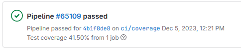
Create Coverage and Pipeline status badge

Research how to add badges to your project and add the coverage and pipeline status badge to your project. You can also add badges for other things if you want to.

Let these badges link to relevant pages in your project.

For the coverage badge to work, the coverage extraction must be setup correctly, see Code Coverage parsing for more information.

Your project's home should look something like this:

Deployment Optimization (GitLab Rules)

As some have noticed, as our pipeline is set up currently changes to any branch will result in a new latest image version and a deploy our kubernetes resources.

This is far from ideal, as branches often contain experimental code that is not ready for deployment. Furthermore, as multiple people are working on separate branches, their deployments will overwrite, and sometimes even break each other.

To avoid this we need to dynamically trigger certain jobs. In GitLab we can use the rules keyword to define rules to trigger jobs. These rules can be very simple or very complex, depending on your needs.

GitLab rules

Each rule has two attributes that can be set.

• when allows you to designate if the job for example should be excluded (when: never) or only built when previous stages ended successfully (when: on_success). Other options are when: manual, when: always and when:delayed.
• allow_failure can be set to true, to keep the pipeline going when a job fails or has to block. A job will block when for example when: manual is set: the job needs manual approval and this will block following jobs.

For each rule, three clauses are available to decide whether a job is triggered or not: if evaluates an if statement (checking either environment variables or user defined variables), changes checks for changes in a list of files (wildcards enabled) and exists checks the presence of a list of files. These clauses can be combined into more complex statements as demonstrated in the example below.

rules:
  - if: '$CI_PIPELINE_SOURCE == "merge_request_event"'
    when: manual
    allow_failure: true
  - if: '$CI_COMMIT_BRANCH == "master"'
    changes:
      - Dockerfile
    when: on_success
  - if: '$CI_PIPELINE_SOURCE == "schedule"'
    when: never

Disclaimer: the above snippet makes no sense and is merely here to illustrate how the rules work and are evaluated.

The first rule will trigger a manual job, requiring a developer to approve the job through GitLab, if the source of the pipeline is a merge request. Failure is explicitly allowed so the following jobs and stages aren't blocked by this job. The second rule will trigger for changes of Dockerfile (on the root level of the repository) on the master branch. When previous stages fail, this job will be skipped because of when: on_success, which dictates to only trigger a rule upon successful completion of previous stages (this is also the default). The third and final rule will exclude this job from being triggered by Scheduled pipelines through when: never.

For full documentation on the rules keyword see official GitLab CI/CD docs, it has extensive examples to get you started. For a list of all default environment variables to check via the if statement visit this page.

Warning

Before introducing the rules keyword into GitLab CI/CD, only|except were used to define when jobs should be created or not. The rules syntax is an improved and more powerful solution and only|except has been long deprecated.

Avoiding unnecessary deployments

The simplest strategy to solve our problem is to limit deployment and creation of the latest tag to the default branch only. Controlling when jobs and pipelines get run is done through GitLab rules keyword.

Use Predefined Variables

GitLab provides many predefined variables that make your pipeline more flexible and maintainable. Instead of hardcoding branch names like main or master, use $CI_DEFAULT_BRANCH which automatically refers to your repository's default branch.

This makes your pipeline: - Resilient to branch naming changes (main vs master) - Portable across repositories with different default branches - Following DevOps best practices (avoid hardcoding!)

Example:

rules:
  - if: $CI_COMMIT_BRANCH == $CI_DEFAULT_BRANCH  # Good!
  # - if: $CI_COMMIT_BRANCH == "main"           # Avoid hardcoding!

See GitLab Predefined Variables for the full list.

Set up rules

Set up your pipeline with rules so they at the least do the following:

• Only push the latest tag when the pipeline is run on the default branch
• Do not deploy the latest build to the cluster, unless the pipeline is run on the default branch
• Make sure that your full pipeline runs when committing a tag to the repository such as Lab 4

You can add rules that expand on this strategy, to e.g. deploy certain feature branches through a manual trigger or limit building of code to when it has actually changed, if wanted. Start with the required rules and expand if needed. Include your overall strategy in your report and make sure that your final pipeline functions as expected.

Reliability & Resilience (Chaos, Persistence, Shutdown)

Chaos Engineering

Chaos Engineering is the discipline of experimenting on a system in order to build confidence in the system’s capability to withstand turbulent conditions in production. It brings about a paradigm shift in how DevOps teams deal with unexpected system outages and failures. Conventional Software Engineering teaches us that it is good practice to deal with unreliability in our code, especially when performing I/O (disk or network operations), but this is never enforced. There are many stories of large systems fatally crashing because engineers e.g. never imaged two services failing in quick succession.

In Chaos Engineering, failure is built into the system, by introducing a component that can kill any service at any time. This changes your psyche as a Developer or DevOps engineer: failure is no longer an abstract concept that will probably never happen anyway. Instead, it becomes a certainty, something you have to deal with on a daily basis and keep in the back of your head for any subsequent update you perform on the codebase.

Context

Chaos Engineering was pioneered at Netflix as part of a new strategy for dealing with the rapid increasing popularity of the streaming service, causing significant technical challenges with regards to scalability and reliability.

For the Devops Game, we implemented a lite version of Chaos Engineering. There is a component in place that can kill logic-service pods, but it does not operate in a completely random way. To keeps things fair, the component targets Teams in a uniform way by cycling through a shuffled list of the participating Teams. The logic-service pod for each Team will be killed a fixed number of times during each game session.

Remember: Kubernetes is declarative in nature and uses a desired state, meaning if you specify that a deployment should have one pod (using the spec.replicas attribute), Kubernetes tries to make sure that there is always one pod running. As a result, the pod for your logic-service will automatically restart each time it is killed by our Chaos component, so you don't have to worry about that.

However, the operation of your logic could be impacted after a restart. Especially if you rely on building up a model of the game world in memory for guiding your decisions. In the next section, we will discuss how you can persist and recover important parts of your state.

Saving & Restoring state

GameState

You can extend your Logic Service with functionality to periodically save your in-memory state, with the goal of being able to restore this state when your service is restarted.

An easy way to save your state is by using the Jackson serialization library. Using Jackson, you can convert any POJO (Plain Old Java Object) into a JSON string, which can be written to a file.

Note

We recommend encapsulating all your game state into a new Java class. This class should contain nothing but your game state properties as private fields (with public getters and setters) and a generated hashCode and equals function. This helps to create a straightforward flow for saving and restoring your state.

Example of a simple GameState class:

package be.ugent.devops.services.logic.persistence;

import be.ugent.devops.services.logic.api.Location;

import java.util.HashSet;
import java.util.Objects;
import java.util.Set;

public class GameState {

    private String gameId;

    private Set<Location> resources = new HashSet<>();
    private Set<Location> enemyBases = new HashSet<>();

    public String getGameId() {
        return gameId;
    }

    public void setGameId(String gameId) {
        this.gameId = gameId;
    }

    public Set<Location> getResources() {
        return resources;
    }

    public void setResources(Set<Location> resources) {
        this.resources = resources;
    }

    public Set<Location> getEnemyBases() {
        return enemyBases;
    }

    public void setEnemyBases(Set<Location> enemyBases) {
        this.enemyBases = enemyBases;
    }

    public void reset(String gameId) {
        this.gameId = gameId;
        resources.clear();
        enemyBases.clear();
    }

    @Override
    public boolean equals(Object o) {
        if (this == o) return true;
        if (o == null || getClass() != o.getClass()) return false;
        GameState gameState = (GameState) o;
        return Objects.equals(gameId, gameState.gameId) && Objects.equals(resources, gameState.resources) && Objects.equals(enemyBases, gameState.enemyBases);
    }

    @Override
    public int hashCode() {
        return Objects.hash(gameId, resources, enemyBases);
    }
}

It is important that GameState has a reset method, which is able to clear all the state attributes, e.g. when a new game is started!

You could embed an instance of this class in your FactionLogicImpl to keep track of resource locations or enemy bases, so you can use this information for making informed decisions in controlling your units. To make an instance of GameState available in FactionLogicImpl, you can rely on the Quarkus CDI framework, by providing a Producer method which creates an instance by reading a JSON file which contains the previously written state:

package be.ugent.devops.services.logic.persistence.impl;


import be.ugent.devops.services.logic.persistence.GameState;
import be.ugent.devops.services.logic.persistence.GameStateStore;
import io.quarkus.logging.Log;
import jakarta.inject.Inject;
import jakarta.inject.Singleton;

public class GameStateInitializer {

    @Inject
    GameStateStore gameStateStore;

    @Produces  // Declare as Producer Method
    @Singleton // Make sure only one instance is created
    public GameState initialize() {
        Log.info("Fetching initial game-state from store.");
        return gameStateStore.read();
    }

}

This GameStateInitializer relies on an implementation of GameStateStore, who's interface is declared as follows:

package be.ugent.devops.services.logic.persistence;

public interface GameStateStore {

    void write(GameState gameState);

    GameState read();

}

Implement GameStateStore

Provide an implementation for this interface. Write will have to encode the GameState to JSON then save it to a file. Read will have to read the JSON file and decode it to a GameState object. Check the io.vertx.core.json.Json package which is bundled in the Quarkus framework for help with encoding and decoding JSON. For reading and writing files, you can use the java.nio.file package.

Some further pointers:

• Annotate the class with @ApplicationScoped, so it can be injected in GameStateInitializer (and your FactionLogicImpl, see next section).
• Make the path to the folder that is used for storage configurable (see the Quarkus guide on configuring your application). Name this configuration property game.state.path.
• The actual filename can be static, e.g. gamestate.json
• Prevent unnecessary file writes: when the GameState has not been modified, skip the write operation. You can implement this by storing the hashcode of the last written GameState in a variable and comparing this value at the start of the write method.

Integration in FactionLogicImpl

You can now integrate a persistent GameState by replacing the following code block in the method nextBaseMove, make sure to inject the necessary fields so they are properly initialized:

if (!input.context().gameId().equals(currentGameId)){
    currentGameId=input.context().gameId();
    Log.infof("Start running game with id %s...",currentGameId);
}

With the following code:

if (!input.context().gameId().equals(gameState.getGameId())) {
    gameState.reset(input.context().gameId());
    Log.infof("Start running game with id %s...", gameState.getGameId());
}

// Trigger write state once per turn
gameStateStore.write(gameState);

This will make sure that GameState is reset when your logic detects that a new game has been started and that the latest GameState is persisted once every turn.

Warning

Remember that our Game server will cancel baseMove or unitMove requests after a timeout of one second. Take this into account when calling your save state method and be mindful of the amount of data you are writing to disk. Monitor your move operations response times using Prometheus instrumentation to gain insight in how much headroom you have left!

Use GameState in your logic

Integrate the GameState in your logic, by replacing any fields and references in FactionLogicImpl that were used to track Game specific data, with new attributes in the class GameState.

Important: do not forget to update the equals() and hashcode() when modifying attributes.

Handle controlled shutdown

The Quarkus framework supports hooks that enable specifying what code should be executed when the application receives a "sigterm" (termination signal), e.g. when Ctrl + C is entered in the shell executing the application. This allows you to implement controlled shutdown behaviour. The following code sample shows an example of such a hook:

import io.quarkus.runtime.ShutdownEvent;
import jakarta.enterprise.context.ApplicationScoped;
import jakarta.enterprise.event.Observes;
import jakarta.inject.Inject;

@ApplicationScoped
public class ShutdownHook {

    public void onStop(@Observes ShutdownEvent event) {
        Log.info("Shutdown hook triggered - saving game state...");
        // Execute shutdown behaviour here...
    }

}

Handle termination

Add a shutdown hook that saves the GameState to file before allowing the application to terminate.

Required: Include a log statement at the start of your shutdown hook to verify it's being called.

Kubernetes Persistent Volumes

In the section on Grafana persistence, we've briefly touched on the concept of Kubernetes Persistent Volumes and Persistent Volume Claims.

Using the same principles, you can make sure that the game state file you write in your Logic Service code, is still there whenever your service restarts.

First, you need to add a PVC resource file volumeClaim.yaml to your k8s folder, with the following contents:

kind: PersistentVolumeClaim
apiVersion: v1
metadata:
  name: logic-service-pvc
  labels:
    app: logic
spec:
  storageClassName: k8s-studstorage
  accessModes:
    - ReadWriteOnce
  resources:
    requests:
      storage: 100Mi

This file describes the PersistentVolumeClaim, declaring that it should use the k8s-studstorage storageClass and reserve 100 mebibyte (which should be more than sufficient to store your state).

You will need to configure your deployment and logic service container to use this volume. Check out the official docs to find out how use claims as volumes.

setup volume provisioning

Add the necessary config to your deployment.yaml to start using the PersistentVolumeClaim.

See https://kubernetes.io/docs/concepts/storage/persistent-volumes/#claims-as-volumes.

Make sure to update your Logic Service configuration: the path used for the volume mount should be the same as the path set for the variable game.state.path (or GAME_STATE_PATH when supplying a value using environment variables).

Advanced Topics (Zero-Downtime & Alerting)

The following sections cover advanced topics that are essential for production-ready services but require independent research and problem-solving. These practices are widely used in the industry to ensure high availability and reliability.

Zero-Downtime Deployments (Probes & Rolling Updates)

When you deploy a new version of your Logic Service, there's typically a brief period where the service is unavailable. In production environments, this downtime can impact users and disrupt operations. Zero-downtime deployments ensure your service remains available even during updates.

Health Checks

Kubernetes provides health probes to ensure your pods are functioning correctly:

• Liveness Probe: Determines if the application is running properly. If it fails, Kubernetes restarts the pod (e.g., detect deadlocks, hung threads).
• Readiness Probe: Determines if the application is ready to serve traffic. If it fails, Kubernetes removes the pod from service endpoints until it passes.

For zero-downtime deployments, readiness probes are critical. They ensure that:

1. New pods are fully initialized before receiving traffic
2. Old pods are removed from the load balancer before being terminated

We will not use startup probes - your Logic Service starts quickly enough that properly configured liveness and readiness probes are sufficient.

Implementing Health Checks in Quarkus:

Quarkus provides health check support via SmallRye Health. Add the extension to your pom.xml:

<dependency>
    <groupId>io.quarkus</groupId>
    <artifactId>quarkus-smallrye-health</artifactId>
</dependency>

This automatically exposes health endpoints:

• /q/health/live - Liveness checks
• /q/health/ready - Readiness checks

For this lab, focus on implementing a custom readiness check. The default liveness check (basic HTTP response) is sufficient.

Practical Health Check Ideas

Readiness Check:

Check that your service is ready to handle game logic requests:

• Game State Storage accessible: Verify the PersistentVolume is mounted and writable (important when using state persistence)
• Configuration loaded: Check that required config properties are available
• Dependencies available: Verify injected beans are properly initialized

Example: Check if the game state directory exists and is writable before accepting traffic. This prevents errors when the volume isn't mounted yet.

Liveness Check:

The default Quarkus liveness check (basic HTTP response) is often sufficient. Only add custom logic if you have specific failure modes to detect:

• Thread not deadlocked: Application can execute basic logic without hanging
• Request processing: Track timestamp of last successful request processing - if too old, might be deadlocked

What NOT to check in liveness: - Don't check external dependencies (database, APIs) - that belongs in readiness - Don't check resource limits - Kubernetes handles OOMKills automatically - Keep it simple - complex checks can cause false positives

Configure Probes in deployment.yaml

Configure the probes with appropriate timing for your application:

containers:
  - name: logic-service
    livenessProbe:
      httpGet:
        path: /q/health/live
        port: 8080
      initialDelaySeconds: 30
      periodSeconds: 10
      timeoutSeconds: 3
      failureThreshold: 3
    readinessProbe:
      httpGet:
        path: /q/health/ready
        port: 8080
      initialDelaySeconds: 10
      periodSeconds: 5
      timeoutSeconds: 3
      failureThreshold: 3

These are starting values - you must tune them for your application!

Key parameters to understand and adjust: - initialDelaySeconds: How long to wait before first check - periodSeconds: How often to check - timeoutSeconds: How long to wait for response - failureThreshold: How many failures before taking action

Required: Tune Your Probes

The default values above will NOT be optimal for your application! You must:

1. Observe your application's behavior:

   • Monitor pod startup: kubectl describe pod <pod-name>
   • Watch events: kubectl get events --sort-by='.lastTimestamp'
   • Check logs: kubectl logs <pod-name>

2. Measure actual timings:

   • How long does your app take to start?
   • How quickly does it respond to health checks?
   • Does it need more time under load?

3. Adjust probe settings accordingly:

   • Too aggressive → false positives and unnecessary restarts
   • Too lenient → slow recovery and longer downtime
   • Find the balance for YOUR application

4. Test during deployments:

   • Does zero-downtime work with your settings?
   • Are pods ready before receiving traffic?
   • Do old pods shut down gracefully?

Research probe configuration best practices - understand the trade-offs between startup time, detection speed, and reliability.

Document in your report:

• Final probe settings and why you chose them
• How you tested and validated your configuration
• Trade-offs you considered

Research Resources

• Quarkus SmallRye Health Guide - Complete guide with examples
• Kubernetes Health Probes - Kubernetes documentation
• Pod Lifecycle - Understanding probe behavior

Rolling Updates

Kubernetes Deployments support rolling updates by default, but proper configuration is needed to achieve true zero-downtime:

• maxSurge: How many extra pods can be created during the update
• maxUnavailable: How many pods can be unavailable during the update
• minReadySeconds: Minimum time a pod should be ready before being considered available

Implement Zero-Downtime Deployments

1. Implement a custom readiness check (required) - verify your service is truly ready (e.g., storage accessible, dependencies initialized)
2. Optionally implement custom liveness check if you have specific failure modes to detect beyond default HTTP response
3. Configure probes in deployment.yaml - start with suggested values, then tune based on your observations
4. Configure rolling update strategy to ensure zero downtime (maxSurge, maxUnavailable)
5. Test your deployment by:
   • Starting a game session
   • Deploying a new version during the game
   • Verifying the game continues without interruption
   • Monitoring pod events for probe failures
6. Document your configuration choices and test results in your report
   • Verifying the game continues without interruption

Alerting

Monitoring data is only valuable if you act on it. Alerts notify you when metrics indicate problems or abnormal behavior.

Grafana Alerting

Grafana provides built-in alerting that can evaluate your metrics and send notifications when thresholds are exceeded. Modern Grafana versions use a unified alerting system that's powerful but requires some learning.

Alert Targets: GitLab Alerts Integration

GitLab has a built-in Alerts feature designed for incident management. You can send alerts from Grafana directly to GitLab using webhooks!

Recommended Approach: GitLab Alerts

1. Enable GitLab Alerts in your project:

   • Go to your GitLab project → Settings → Monitor → Alerts
   • Create a new HTTP integration
   • Copy the webhook URL and authentication token

2. Configure Grafana Contact Point:

   • In Grafana: Alerting → Contact points → New contact point
   • Type: Webhook
   • URL: Paste your GitLab Alerts webhook URL
   • HTTP Method: POST
   • Add the authentication token in an Authorization header (Bearer token)

3. View alerts in GitLab:

   • Monitor → Alerts shows all fired alerts
   • Each alert creates an entry with timestamp and details
   • Supervisors can easily verify your alerting is working
   • You can map the alert payload fields in Grafana to GitLab alert fields for better context, see GitLab docs.
   • In order to have automated resolving you will need to ensure the alert start time, end time and fingerprint fields are mapped correctly!

Documentation: GitLab Alerts Integration

Implement Alerting

Define at least 2 meaningful alerts for your Logic Service. Choose alerts that help you monitor your service's health and performance.

Alert suggestions:

• Memory approaching limit: Alert when memory usage > 80% of your configured limit
• High move execution time: Alert when average move time exceeds threshold (e.g., >500ms risks timeouts)
• Error rate spike: Alert when error count increases significantly
• Game state changes: Alert on game start/end for lifecycle monitoring
• Pod availability: Alert when deployment has 0 ready replicas
• Resource starvation: Alert when gold balance critically low for extended period

Requirements:

1. Configure alerts in Grafana with appropriate thresholds and evaluation intervals
2. Set up notifications to GitLab Alerts (recommended)
3. Generate alert activity - Your GitLab Alerts page must show triggered alerts:
   • Trigger at least one alert manually (e.g., purposefully exceed threshold)
   • OR choose low thresholds that will naturally trigger during testing
   • Ensure there is content for supervisors to review
   • Escalate at least one of these alerts to create a GitLab Incident!
4. Document in your report:
   • Alert configurations with thresholds and why you chose them
   • Screenshots of alerts firing in Grafana
   • Link to a GitLab Incident created from one of your triggered alerts
   • How you would respond to each alert type in production

Making Alerts Trigger for Testing

Your GitLab Alerts page must have some activity to prove your alerting works. Strategies:

• Purposeful triggering: Set low thresholds temporarily (e.g., memory > 50% instead of > 80%), run a game, then adjust to production values
• Game lifecycle alerts: Alert on game start/end - guaranteed to trigger during testing

The goal is demonstrating your alerting pipeline works end-to-end, not just showing configuration!

GitLab Alerts Configuration

Map alert fields correctly for better alert details and auto-resolution:

• Start time: ${values.A.Labels.__alertId__} or similar timestamp field
• End time: Configured for resolution
• Fingerprint: Unique alert identifier for deduplication

See GitLab alert field mapping for details.

Research Starting Points:

• Grafana Alerting Documentation
• GitLab Alerts Integration

Practicalities & Checklist

This lab must be completed before Monday, 8 December at 23:59.

Warning

All support outside the physical Lab session is handled via the GitLab Issue tracker! Do not expect support outside of the normal office hours.

Checklist

Core Requirements

• Monitoring & Observability
  • Deploy Grafana using Helm, add configuration to monitoring/grafana-values.yaml
  • Create Grafana admin secret with keys admin-user and admin-password
  • Test metrics locally with Docker Compose before deploying
  • Create enhanced resource dashboard with CPU/Memory request/limit lines and percentage stats
  • Create at least 4 custom metrics (move_execution_time and 3 others)
  • Create move_execution_time dashboard with histogram visualization
  • Create dashboards for your other custom metrics
  • Document metrics and dashboards in monitoring/instrumentation.md

• Pipeline Quality & Visibility
  • Add code coverage reports to unit test job
  • Parse coverage with GitLab (shows in MRs, job details, history)
  • Add unit test reports to pipeline overview
  • Achieve at least 60% code coverage
  • Add pipeline status and coverage badges to README

• Deployment Optimization
  • Configure resource limits in deployment.yaml (256-512 MiB memory, 100m CPU request)
  • Set up GitLab CI rules: push latest only on default branch, deploy only on default branch
  • Configure full pipeline trigger on tag push (e.g., Lab 4)

• State Persistence & Reliability
  • Implement GameStateStore to save/load state to JSON file
  • Use GameState in logic to track and persist game information
  • Add shutdown hook to save state before termination
  • Configure Persistent Volume usage in deployment.yaml

Advanced Challenges (Optional)

• Zero-Downtime Deployments
  • Add SmallRye Health extension to project
  • Implement custom readiness check (e.g., storage accessible)
  • Optionally implement custom liveness check
  • Configure probes in deployment.yaml with tuned timing
  • Configure rolling update strategy (maxSurge, maxUnavailable)
  • Test zero-downtime during active game session

• Alerting
  • Define at least 2 meaningful alerts in Grafana
  • Configure GitLab Alerts integration (Settings → Monitor → Alerts)
  • Trigger alerts to generate activity in GitLab Alerts page
  • Document alert configurations and thresholds
  • Include screenshots of alerts in GitLab Monitor → Alerts

Submission

• Add a tag¹ Lab 4 to the commit you consider the final result of this lab session.
• Create an issue Lab 4 Report, labeled with Report & Lab 4 , and add a concise report containing:
  • Link to the pipeline run for your Lab 4 tag
  • Add a changelog for your Faction Logic implementation: what was added, fixed, removed. Link to the corresponding issues
  • For advanced challenges: include evidence (screenshots, logs, configuration) demonstrating functionality

---

1. You can tag on Gitlab: use the tab "Repository" (left menu), click "Tags" , then "New Tag". You can also tag using git directly: https://git-scm.com/docs/git-tag. ↩